April 2022 — This section provides techniques for identifying market opportunities for selected retail and service retail business categories. It examines business opportunities in terms of number of businesses the market could bear, total sales, and square feet of occupied business space. Other more qualitative and equally important market considerations are also discussed in this section. A selection of tools to measure demand and supply are presented.

Demand & Supply Analysis

Once you have assembled sufficient information on the trade area, you’re ready to focus on a detailed analysis of business opportunities by specific category. You have learned it is imperative to fill vacancies with viable businesses and to give residents access to necessary retail goods and services. You want to support your work with data and solid analysis to help ensure the success of these businesses.

In this section we focus on those retail and service businesses that commonly have a storefronts in downtown districts. This includes traditional retail stores such as pharmacies and groceries, but also services such as auto repair and hair salons. The analysis of retail and service business opportunities involves both quantitative examination and qualitative insight following a three-step process:

• Assess demand;
• Inventory supply; and
• Draw realistic conclusions.

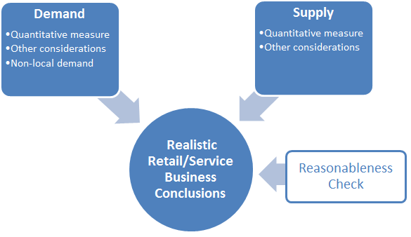
To help you with the quantitative aspects of this process, this section provides various tools, ranging from simple to complex, that can be used for one or multiple business categories. A quantitative demand and supply comparison is important because it helps put numbers behind your analysis and gives you some measures to support your business development activities. However, as the analysis is as much an art as a science, your study must also consider numerous qualitative factors. The following chart illustrates factors that go into an evaluation of retail and service business opportunities.

Definitions Used in this Section: NAICS: The North American Industry Classification System is used by the federal government for classifying all businesses and their related statistics. Each business is classified by a NAICS code and a specific store category.  For example, 44211 is the code for furniture stores.  Descriptions of 71 selected retail and service business categories used in this section are available here.

Demand: In market analysis, demand is the amount of a good or service required to fulfill the needs of customers in your area. This is mainly driven by the size of your trade area, the number of customers in your trade area, and their purchasing power. This is often calculated by NAICS category. Demand can be measured in square feet, number of stores, or total sales.

Supply:  In market analysis, supply is the amount of a good or service currently distributed in the marketplace. This is often organized by NAICS category and can be measured in square feet, number of stores, or total sales. The data that is available to you and the ease of collecting this information determine how you measure supply in your community.

Note: Another way to analyze the retail market is to estimate spending by product type. Data is available from the U.S. Bureau of Labor Statistics as well as private data firms that can be used with local demographic data to estimate local demand. However, it is often difficult to` estimate a comparative “supply” figure. Nevertheless, for certain categories, a demand and supply analysis by product type may be appropriate.

Return to top

Step 1: Assess Demand

In market analysis, demand is the amount of a good or service required to fulfill the needs of customers in your area. The spending potential of trade area residents typically determines most of the demand for local retail goods and services. This demand can be modeled using various quantitative measures. You must also consider other qualitative measures to more fully understand characteristics of your local market and of non-local consumers who may shop in your community.

Market Potential Method

This method for determining market potential estimates total demand for retail and services businesses in a trade area based on historic customer spending patterns. From secondary data sources like the U.S. Economic Census, you can obtain reliable data to estimate domestic sales per capita and average sales per store. You can use this information to estimate demand by store type. Market potential can express demand in total sales, number of businesses, or square feet of retail space (also known as gross leasable area, or GLA). Tools in this section such as the  Gap Analysis Calculator (Tool 2),  Pull Factors (Tool 3), and the Trade Region Gap Analysis (Tool 4) can be used to calculate market potential and business gaps for your trade area.

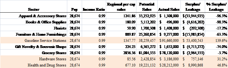
“Potential sales” are estimated sales that could be achieved if all people living within a trade area only shopped within the trade area. Actual (or estimated) sales are compared to potential sales to determine a “surplus” or “leakage.” If actual sales exceed potential sales, a sales surplus exists. A surplus implies either that (a) people travel from outside the trade area to area or (b) people living within the trade area consume more than would be typically expected given their income levels. However, if actual sales are less than potential sales, the trade area suffers a sales leakage. A leakage indicates that either (a) people living within the trade area shop outside the county or (b) people living within the trade area consume less than would be expected given their income levels.

Other Local Demand Considerations

Examining local demand in terms of numbers and dollars is only part of the analysis. There are also a number of important qualitative considerations to help you gauge the depth of trade area demand and your downtown’s ability to capture it. These are discussed in other sections of the toolbox and include:

• Consumer Perceptions and Behavior. What have you learned from local research about consumer perceptions and behavior related to downtown business activities? Has a sidewalk intercept study been conducted to assess your district’s strengths and weaknesses? Has a survey been conducted to learn why some people never come downtown? Use findings from business owner surveys, consumer surveys, and focus group sessions as described earlier in the toolbox.
• Demographic and Lifestyle Characteristics. Does data on age, income, home ownership, and lifestyle segmentation indicate that local residents are more likely to purchase goods within a particular store category?  Use findings from your analysis of market demographics and lifestyles as described earlier in the toolbox.
• Economic Conditions. The overall health of the local and regional economy should be considered as it indirectly impacts local demand.  Do trends in the labor force, major employers, unemployment, street/highway traffic, and quality of life contribute to increased market demand for retail and services?  Use findings from your analysis of local and regional economic conditions as described earlier in the toolbox.

Estimating Non-Local Demand

While demand and supply analysis typically focuses on residents of the trade area, many communities also depend on non-local demand to support local businesses. These consumer segments can include:

• Tourists and visitors;
• Second homeowners; and
• In-commuters (those who travel regularly into your area to work).

Findings from business owner surveys, consumer surveys, and focus group sessions that include questions about non-local market segments can provide valuable insight regarding non-local demand. In addition, some communities conduct research specific to these market segments such as visitor intercept surveys, second-home owner geo-demographics analyses of their place of origin, and in-commuter paycheck surveys.

Return to top

Step 2: Inventory Supply

In a market analysis, supply is the amount of a good or service available for sale in the trade area. To analyze supply, a database of existing businesses must be constructed for each store category examined. The database of NAICS store categories should include all of the retail businesses within the trade area (the geographic area that was used to calculate demand).

Quantitative Measures

As noted, your database should include all current retailers in the trade area. Information on each business should include:

• Name of business;
• Address;
• Estimated sales range (if available); and
• Estimated store size (in square feet).

There are a two ways to build your inventory of current supply—through secondary data and through a locally generated database.

Secondary Data

The simplest method for building your inventory is to purchase a list of businesses from a national data provider. A number of national firms compile this information from Yellow Page listings, annual company reports, and other sources. Purchasing a list can be expensive depending on the number of businesses in your trade area. While some sources provide sales estimates per establishment, they typically do not include store size (square feet)—a useful method in comparing demand and supply. Further, the data may not be sufficiently accurate as there are often errors in store category coding, location, business status, etc.  You must take care to properly examine purchased lists for accuracy and fix any errors.

Locally Generated Database

A second and often better option for assessing supply is to develop your own database. Certainly this is a time-intensive process, although it provides the most current and accurate information. Local databases are often compiled through walking or driving tours of downtown and/or trade areas. While collecting sales estimates will be nearly impossible using this method, it is possible, with a little practice, to estimate store size (see Estimating Store Size exhibit). The building and business Inventory described earlier in the toolbox can be used to record this data.  Also, if your city has a GIS department it is possible they have building footprint data that could be used to estimate size.

Estimating Store Size

Gross leasable area (GLA) can be estimated by actually measuring a building’s street-front width and estimating its depth.  Square feet can be estimated by comparison with other stores.

Other Supply Considerations

Qualitative factors should also be part of the supply analysis. For each NAICS retail category, consider:

• Presence of a Market Niche. Are there clusters of businesses in a store category that have created a critical mass of activity and a distinct market niche for the business district? For example, a cluster of home improvement stores may not represent oversupply in the market if together they have created a destination.
• Position Relative to Other Business Districts in the Trade Area. Most communities contain multiple business districts. These may include malls, strip centers, commercial corridors, neighborhood centers, and more. The supply analysis must recognize that downtown may not be the ideal location for all store categories.
• Retail Vitality Relative to Other Downtowns. What is the retail supply in this category in other peer city downtowns? Are the selections of specialty retail in your downtown as interesting and exciting as those in other places? Use findings from your peer city comparison analysis section of the toolbox.
• Competitiveness of Existing Stores in the Trade Area. Are existing downtown stores in this category providing the merchandise and service that local shoppers demand?  Is the category already present in the district and is it thriving?  Are the stores chains or independents? Use findings from business owner surveys, consumer surveys, and focus group sections of the toolbox.
• Competitiveness of Existing Stores outside the Trade Area. Do surrounding communities with regional shopping centers and big box stores siphon business in this category out of the trade area? Use findings from business owner surveys, consumer surveys, and focus group sections of the toolbox.

Return to top

Step 3: Draw Realistic Conclusions

The final step reconciles information gathered in the first two steps in an effort to identify realistic business expansion and recruitment opportunities. For purposes of this toolbox, these opportunities are identified as specific business categories where demand exceeds supply.

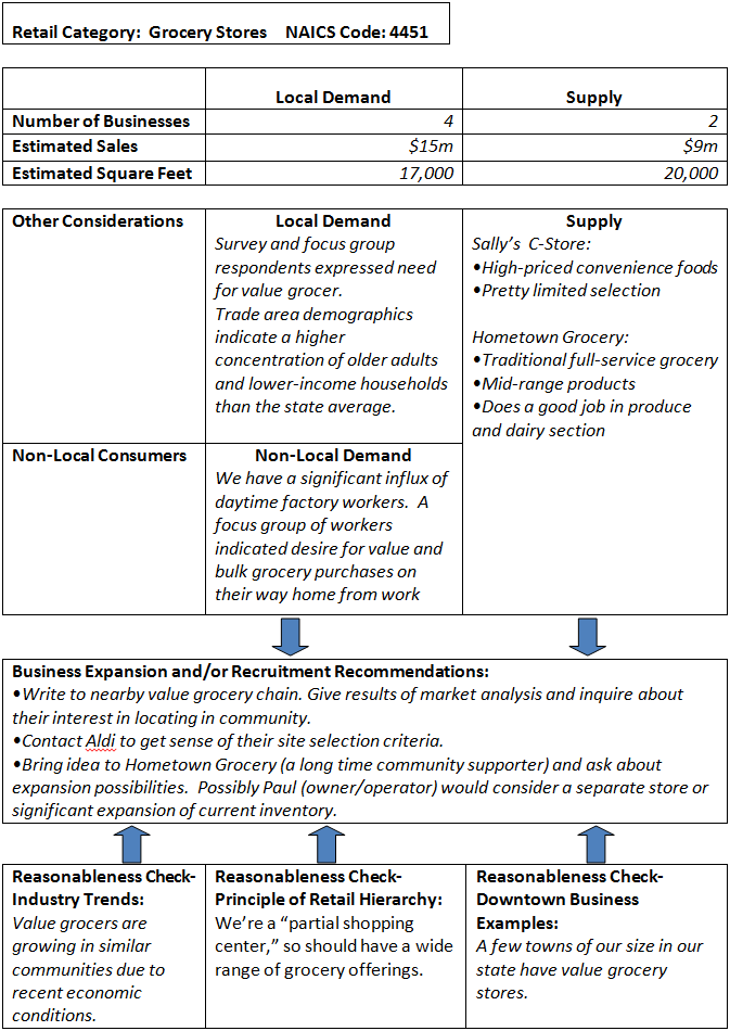
Realistic expectations are important so that business development initiatives lead to achievable outcomes. The Retail and Service Business Opportunities Worksheet that follows can be used to summarize your analysis for each of the business categories being studied. Given the amount of information that must be gathered, we suggest completing this worksheet for high-prospect categories only.

Worksheet Instructions

1. Record the retail category and corresponding NAICS code.
2. Use one or more of the quantitative tools presented later in this section to help you calculate and record demand and supply. The purpose here is to determine if demand significantly exceeds supply, a signal that there may be business development opportunities. These tools, which vary in complexity, can help you measure demand and supply according to number of businesses, estimated sales, or estimated square feet.  They include:
   • Business Mix Analysis. A derivation of “threshold analysis,” this tool helps you compare the number of businesses in your downtown with other similar-sized communities.
   • Gap Analysis Calculator. This tool allows you to calculate trade area consumer spending and potential demand in terms of estimated sales, number of stores and square footage—then compare each with actual levels.
   • Pull Factors. Pull factors can be used to measure the relative strength of the local retail market and whether or not it is drawing in sales from other communities.  This tool does not necessarily represent the trade area, as it is based on political boundaries.
3. Record other considerations pertinent to the local trade area consumer. This information may come from surveys, focus groups, or demographic and lifestyle analyses. These considerations should provide additional insight on local consumer behavior and competition.
4. Record non-local consumer research findings that describe consumers who may shop in your community, but permanently reside elsewhere. They may include visitors, second homeowners, and in-commuters.
5. Based on the above, develop and record business expansion and/or recruitment recommendations. The quantitative comparison of retail demand with supply provides an initial measure of market opportunities. If there is a significant amount of unmet demand, there may be opportunities for existing businesses to expand or for the community to recruit new businesses. Business development opportunities also may exist in areas where supply is greater than demand, but special conditions offer potential. For example, some communities draw customers from outside their trade area by creating a niche market. You should also consider findings from other research on non-local consumers in making recommendations. Recommendations may center on:
   • Best location with regard to visibility, traffic, and complementary businesses, whether chain or independent;
   • Size in square feet;
   • Price points;
   • Expected market segments; or
   • Downtown enhancements needed.

     Your recommendations should highlight business categories that promote a vibrant mix in the district, complement existing businesses, and offer reasonable evidence that an expanded or recruited business will have opportunity for success.

6. Recommendations must undergo a check for reasonableness. In other words, do a reality check. It is important to step back from the analysis and ask if your recommendations are based on actual consumer behavior and business location practices. Consider the following for this business category:
   • Industry Trends. Do businesses of this type locate in downtown districts? Can they co-exist among large-format stores on the edge of town? Click on Industry Links to access trade associations for store- specific research.
   • Principle of Retail Hierarchy. Can your community support this business? Retail hierarchy ranks communities based upon the carrying capacity for certain types of businesses and the distances shoppers are willing to travel.  A downtown may be destined to only serve a minimum convenience market (gas station and grocery store).  Conversely, it might be large enough to offer a complete shopping market with retailers such as book stores, specialty foods and sporting goods. For more information, see the factsheet on Retail Hierarchy.
   • Other Successful Downtown Businesses Examples. Examples of similar businesses that are successfully operating in other downtowns may be helpful. The Innovative Downtown Business Online Clearinghouse provides examples of specific stores that have been recognized as generators of traffic to their respective downtowns.

Retail and Service Business Opportunities – Sample Completed Worksheet

Gap Analysis Calculator

NAICS Categories Analyzed

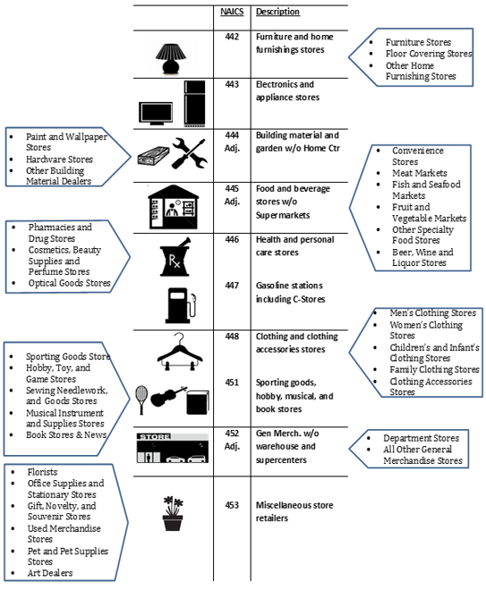
This analysis provides an estimate of demand and supply in the Downtown Study Area for 14 categories of retail and eating/drinking places.  Most of these categories are presented at the three-digit NAICS level. The categories used (see following illustration) reflect the types of businesses found in many Downtowns. Again, various categories are adjusted to exclude large format stores including home centers, supermarkets, warehouse clubs and supercenters.

Geographic Definitions

The Downtown Study Area used in this analysis represents the central area of concentrated commercial activity.  It is often defined by a Business Improvement District or Main Street District boundaries.

A Trade Area is the geographic area from which a community generates the majority of its customers. Knowing the size and shape of the Trade Area is important because it allows for measurement of the number of potential “resident” customers and their spending potential.

Market Segments

For many communities, Downtowns can capture spending from three market segments.  These segments include:

1. Residents of the Trade Area
2. Workers of all employers in the Downtown Study Area
3. Visitors including leisure and business travelers to the County

The calculation of demand for these market segments follows.

1. Trade Area Resident Demand

The demand for the subject Study Area is based on a “proportionate share” of the broader Trade Area as defined earlier. Typically, not all categories are represented by the same Trade Area as some stores pull from a larger “destination Trade Area” while others pull from a smaller “convenience Trade Area.”  The subject Study Area will compete for a share of Trade Area demand.

Consumer spending potential for each business category is calculated as in the following drugstore example:

Assumption	Description	Drugstore Example
Population	Number of residents in the Trade Area.	82,616
Spending Per Capita	U.S. sales in store category (per the 2012 US Economic Census) divided by U.S. population.	$867
PCI Index (US= 100)	The per capita income in the Trade Area indexed to the U.S. per capita income (per the most recent US Census).	99
Behavioral Index (US=100)	A local modifier of consumer behavior indexed to the U.S. average consumer. This subjective factor accounts for lifestyle factors that would increase (>100) or decrease (<100) a person’s likelihood to purchase in this business category in the Study Area.	87
Trade Area $Potential	Multiplication of the above variables.	$61,676,000
SA/ TA Establishments	A measure of the current commercial activity based on the number of businesses (or retail square feet) in the Study Area (SA) as a percent of Trade Area (TA). This is also defined as “proportionate share.”	12%
Study Area $Potential	Multiplication of Trade Area $Potential and SA/TA Establishments produces Trade Area resident demand that could reasonably be captured by Study Area businesses based on its proportionate share.	$7,401,000

2. Study Area Worker Demand

Study Area worker demand potential is based on the number of employees in the district, multiplied by office worker spending as estimated by the International Council of Shopping Centers (2012). Sales are then allocated among the retail and eating/drinking place categories in proportion to Trade Area resident spending. A local modifier or behavioral index (US=100) is applied to account for the amount of retail and dining offerings in the subject district relative to other office districts in the country.

Assumption	Description	Drugstore Example
Worker Population	Number of employees in the Study Area. While many are also Trade Area residents, their extensive presence in the district may reflect spending potential over and above that of residents.	3,000
Worker Spending Per Year	U.S. annual sales in store category are based on estimates by the International Council of Shopping Centers (2012).  They are distributed in part according to the 2012 US Economic Census.	$450
Behavioral Index (US=100)	Behavioral Index (US=100) is applied to account for the amount of retail and dining offerings in the subject district relative to other similar size office districts in the country. This is a subjective assumption.	100
Study Area $Potential	Multiplication of the above variables.	$1,350,000

3. Visitor Demand

Overnight and day visitor demand potential is based on your state’s tourism traveler spending estimates for your County.  Sales are then allocated among the retail and eating/drinking place categories in proportion to Trade Area resident spending.  A percent of these sales is allocated to the Study Area based on number of restaurants in the Study Area as a percent of those in the county (SA/Co Estab.). A local modifier, Behavioral Index (Co.=100), is applied to subjectively account for attributes of the Study Area as an inviting place for visitors relative to the county as a whole.

Assumption	Description	Drugstore Example
Annual Visitor Spending-County	Direct annual spending by visitors in county as reported by the State Department of Tourism.  These visitor sales are then distributed in accordance with all sales reported by the 2012 U.S. Economic Census.	$3,904,000
SA/Co. Establishments	A measure of the current hospitality industry activity: the number of eating/drinking places in the Study Area (SA) as a percent of those in the County (Co.).	16%
Behavioral Index (US=100)	Behavioral Index (US=100) is applied to account for attributes of the Study Area as an inviting place for visitors relative to the county as a whole.	125
Study Area $Potential	Multiplication of the above variables.	$781,000

Analyzing the Results

The combined demand from residents, workers, and visitors something represents a realistic attempt to measure spending that could be captured in the Downtown area.  Again, to make the analysis most relevant to Downtowns, it excludes spending at large format stores.

Dividing $Demand by the average sales per U.S. establishment (per the 2012 US Economic Census), results in a rough estimate of the number of stores that can be supported in each business category.  While there are significant limitations in using such averages (sales vary widely among businesses in each category), it does provide a starting point for the comparison of demand with the actual supply of businesses.

Supply is calculated by conducting an inventory of businesses in your Study Area.  Based on demand and supply differences, there may be:

• A shortage of certain business categories Downtown, or
• A concentration of certain businesses that might define a market niche Downtown.

Using the Excel Workbook

An Excel workbook has been developed to calculate sales potential for the 14 retail and eating/drinking place categories.  An illustration of this 11×14” spreadsheet follows.

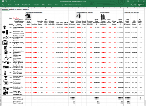
Gap Analysis Calculator

A Surplus-Leakage Method

This tool compares the demand for stores based on the spending potential of your trade area’s residents to the supply of stores actually in your trade area. For a quick introduction to the tool and a basic “how-to” guide, view the video below (video coming soon):

To use the downloadable Trade Area Gap Analysis Calculator (MS Excel Workbook), you need to collect and enter some basic information about your community in an Assumptions worksheet within the Excel Workbook. Information to be entered includes supply of stores by number and/or square foot, local per capita income, and population of trade area.

The workbook formulas are based on available secondary data from the 2007 U.S. Economic Census released in 2010, and the 2008 Urban Land Institute Dollars and Cents of Shopping Centers. Formulas are also based on data about spending patterns from the 2007 Economic Census. The Economic Census provides the most complete and accurate dataset about sales per establishments and per person in the United States. Outputs generated from the calculator can be used as initial estimates of your trade area’s spending potential.

Once your assumptions are entered, click the Report worksheet of the workbook to generate your report. The report will list market demand in sales and square feet for the 71 retail categories.

Assumptions Worksheet

Columns are provided for entering the number of stores and/or square feet of space.  The Assumptions Worksheet also requires entering the name of your trade area, population, per capita income, and U.S. per capita income for the same year.

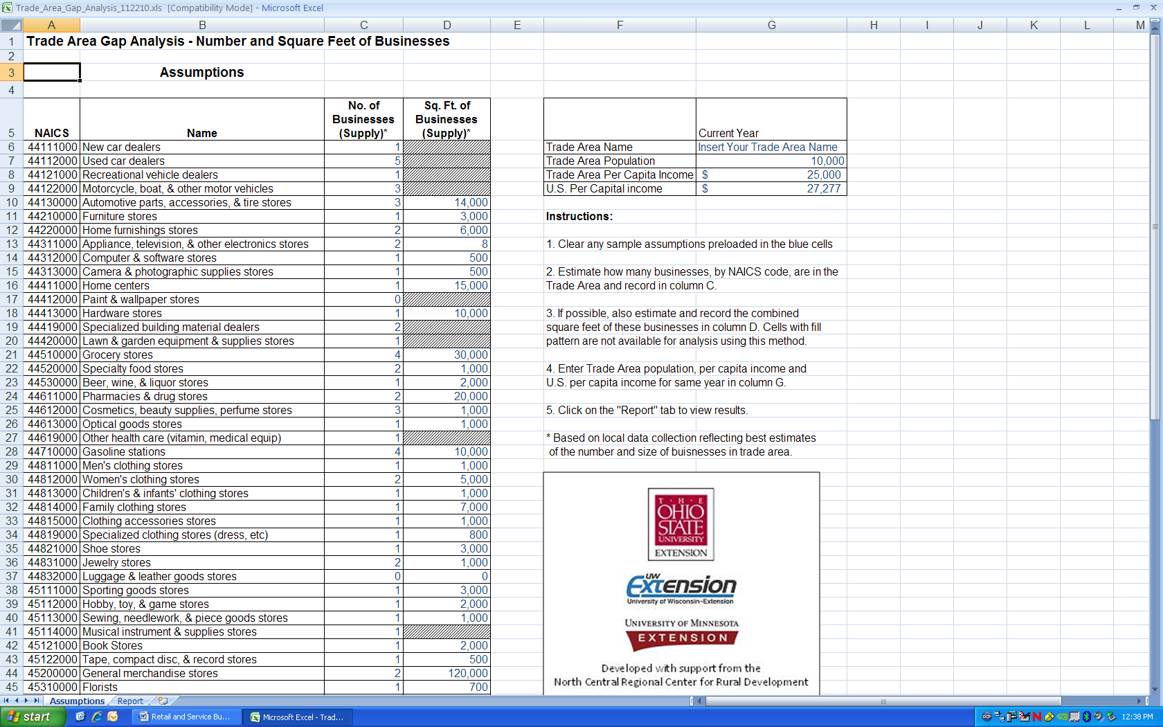
Instructions follow for using the Assumptions Worksheet in the Trade Area Gap Analysis Calculator:

1. Clear any sample assumptions preloaded in the blue cells of the Assumptions Worksheet.
2. Estimate how many businesses, by NAICS code, are in your trade area and record in column C of the Assumptions Worksheet.
3. If possible, also estimate and record the combined square feet of businesses in column D. Cells with the fill pattern are not available for analysis using this method.
4. Enter the trade area population, per capita income and U.S. per capita income for same year in column G.

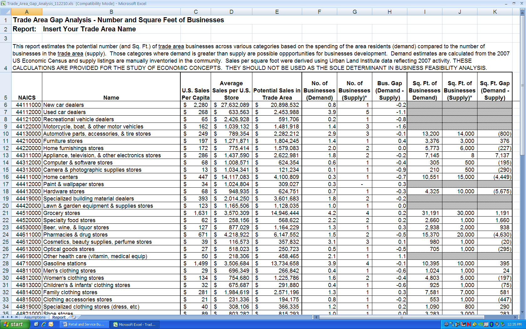
Report Worksheet

Once assumptions are entered, the Report Worksheet generates estimates of trade area demand, supply and any gap (demand less supply) in terms of number of businesses.  For certain business categories (where data is available), data is also provided using square feet of business space as the measure. Specific calculations follow:

• Column C – U.S. Sales Per Capita is equal to the total employer and non
  -employer sales in each business category (according to the 2007 U.S. Economic Census) divided by the U.S. population in 2007 (301.6 million).
• Column D – Average Sales per U.S. Store is equal to total employer and non-employer sales in each business category (according to the 2007 U.S. Economic Census) divided by the number of establishments in that category.
• Column E – Potential Sales in Trade Area is equal to U.S. sales per capita multiplied by the ratio of local trade area per capita income to U.S. per capita income, then multiplied by the trade area population.
• Column F – Number of Businesses (Demand) is equal to potential sales in trade area divided by the average sales per U.S. Store.
• Column G – Number of Businesses (Supply) is based on a business count conducted locally.
• Column H – Business Gap (in terms of number of businesses) is equal to number of businesses (demand) less number of businesses (supply).  A positive gap may be one indicator of opportunities for business expansion or recruitment.
• Column I – Square Feet of Business (Demand) is equal to potential sales in the trade area divided by the average sales per square feet from the 2008 Urban Land Institute’s Dollars and Cents of Shopping Centers.
• Column J – Square Feet of Businesses (Supply) is based on an estimate of actual occupied business space as inventoried locally.
• Column K – Business Gap (in terms of square feet of businesses) is equal to square feet of business (demand) less square feet of business (supply).  A positive gap may be one indicator of opportunities for business expansion or recruitment.

Return to top

Pull Factors

A Surplus-Leakage Method

The pull factor is another important tool of retail trade analysis that will help you answer key questions and identify your community’s economic strengths and weaknesses. The pull factor is a measure of a city, county or regional area’s ability to attract consumers based on its population and statewide average expenditures.

Introduction

“Is our retail marketplace becoming stronger or weaker? Are we losing customers to nearby competitors or are we attracting new customers to our community? Are our sales better than average? “

The answers to these questions are important to your community’s existing and potential retailers. Understanding market performance will help local leaders and development practitioners foster a more conducive environment for retail business development. This also becomes a base for further market analysis that will help current and future business operators make more informed decisions.

Local and regional economic data, as well as these tools of retail trade analysis, will help you analyze your community’s strengths and weaknesses. These tools are not intended to be used in the measurement of specific business or real estate demand and supply analyses, but they are intended to gauge the overall economic health surrounding the business district.

The pull factor—a measure of a community’s or regional area’s ability to attract consumers based on its population and statewide average expenditures— was developed by Ken Stone, Ph.D., and Jim McConnon, Ph.D., at Iowa State University in the 1980s and later refined by numerous economists such as Glen Pulver, Ron Shaffer, and Tom Harris. The pull factor measure is an important part of trade area analysis.

The following examples  are based on Dr. Stone’s definitions and calculations used during his years at Iowa State. As you view pull factor examples from various sources, you will see that they all use similar information but may change the order of calculations, use alternative names for intermediate steps, or determine pull factors as dollars, people, or ratios. The most common modification by economists is the inclusion of the local income index in the pull factor calculation. Dr. Stone did not use the income index until calculating the local sales surplus or sales leakage.  If key stakeholders ask you to explain your economic analysis, this methodology has been easier to demonstrate than others. 

Determining the Pull Factor

As noted, the pull factor is a measure of a community’s ability to attract consumer trade based on its population and statewide average expenditures. It can be used for any trade area for which retail sales are measured whether it is a city, county, or multi-county region. It can also be used for the sum of all retail sales or individual NAICS categories if the state releases such data for local government divisions.  If you are able to obtain data for service businesses, such as restaurants or repair shops, the pull factor analysis can also measure your economic health in those categories.

Calculation Examples

The following examples apply Dr. Stone’s definitions and formulas to Owatonna, Minnesota.  In its simplest form, pull factor is a ratio that equals the “sales per person in a community” divided by the “sales per person in the state.”Following are calculations for furniture sales and overall retail businesses.

Example 12008 taxable furniture sales (NAICS 442) in Minnesota = $1.424 million 2008 Minnesota population = 5.22 million Therefore, Minnesota furniture sales per capita = $1.424 million ÷ 5.22 million = $272 2008 taxable furniture sales in Owatonna = $3.336 million 2008 Owatonna population = 24,855 Therefore, Owatonna furniture sales per capita = $3.336 million ÷ 24,855 = $134 Owatonna pull factor for furniture = Owatonna furniture sales per capita ÷ Minnesota taxable furniture sales per capita Therefore, Owatonna pull factor for furniture = $134 ÷ $272 = 0.49

Example 22008 taxable sales per capita for all retail (NAICS 441-454) in Minnesota = $4,913 2008 taxable sales per capita for all retail in Owatonna = $7,127 Therefore, Owatonna pull factor for retail businesses = $7,127 ÷ $4,913 = 1.45

Interpreting Calculations

A pull factor greater than 1.00 indicates that a community is attracting more customers than its population base. To be sure, some residents do travel elsewhere to make purchases, but more people are coming to this city/county to make purchases than are leaving. If a pull factor is less than 1.00, it indicates that more people are leaving, than entering, the city/county to make purchases.

The simple pull factor calculation demonstrated by the previous examples can be used for any geographic area with existing measures of sales and population, such as cities, counties, and multi-county economic regions. The simple calculation shows how sales are distributed. You can also use this calculation for non-retail businesses, such as restaurants or repair shops.

Comparisons

A pull factor covering a single year in your community is useful. However, you can obtain a better indicator of the health of your retail sector by graphing pull factor over several years for your own community and the communities around you. The graph below shows that a strategy implemented in the late 1990s helped Owatonna outperform other shopping centers in neighboring communities.

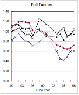
Interpreting Pull Factors

A one-year retail pull factor for a city or county has limited use in an analysis. It does tell you how your community compares to the state average. However, if you have data for different NAICS retail categories, you can start to understand factors that draw people to your community. For example, a longitudinal analysis that covers multi years will give you insight on how important events affected your community’s retail health.

To conduct a longitudinal analysis,  match significant changes in  pull factors with events such as road construction, the opening (or closing) of a store, a natural disaster, the  start of evening store openings, or an economic downturn.

Remember to consider the effect of events in nearby communities, too.  Did a Big Box store open in a community 10 miles away? Did another community begin a loyalty program?  Did a major employer lay off a large number of workers? Once you see how your retail community has fared during significant events you will see how resilient or susceptible your community is to external factors.

Existing businesses and entrepreneurs can also use pull factor data to gain financing for expansion.  As an example, if a community has a strong building materials pull factor, people must be coming to the community to make purchases in that merchandise category.

Business owners can then take a close look to see if they stock a full range of products in the merchandise category with a strong pull factor. Business owners should ask questions such as, “Do we have the latest types of fireplace inserts and accessories?  Do we have tool lines that different types of customers want?  Is there a need for a better quality garden center?”

When interpreting pull factors, you also should take into account political boundaries that may be producing unrealistic results not suitable for comparisons with other communities.  For example, many communities are actually two political entities because a river divides them. Two such examples are Lafayette and West Lafayette, Indiana, and Mankato and North Mankato, Minnesota.

Sometimes a city and bedroom suburb have grown to become one physical entity. The city offers the most shopping, while the suburb is preferred for home ownership.  In essence, the city and suburb act as one business community, but a pull factor analysis for each political entity would show a higher retail pull factor for the city. In cases like this, merge the population and sales data of the city and suburb to produce one community for comparison with others.

Comparing Sales Performance with Expectations

Pull factors are a good measure of how sales are distributed in a state and they enable quick comparisons among communities. But this method does not account for differences in incomes. Dr. Stone developed formulas to obtain this more layered data, as the following examples illustrate.

You would expect people with higher incomes to spend more on retail items. They may simply buy more quantities of retail items or they may buy more expensive items, such as a 50-inch plasma TV versus a 32-inch flat screen variety. With that in mind, you can calculate expected sales in a two-step process. The first step is to calculate the income index based on the following formula:

Income index = Local per capita income ÷ State per capita income

Example 3 2008 Minnesota personal income = $224,670 million2008 Minnesota population = 5.22 million2008 Minnesota per capita income = $43,0402008 Minnesota per capita retail sales = $4, 913 (as calculated in Example 1)2008 Steele County personal income = $1,355 million (Owatonna is in Steele County)2008 Steele County population = 36,5462008 Steele County per capita income ($1,355 million ÷ 36,546) = $37,638Therefore, the income index for Steele County = $37,638 ÷ $43,040 = 0.87

After determining your income index, you can determine expected sales using the following formula:

Expected sales = Local population × State per capita sales × Income index

Example 4 Expected 2008 retail sales for Owatonna = 24,855 × $4,913 × 0.87 = $106,237,975Actual 2008 retail sales were $177,141,585Therefore, the retail sales surplus for Owatonna = $70,903,610 (or 66.7 percent above expected sales). That equates to 16,578 more people shopping in the city (or 66.7 percent above the Owatonna population).

Advanced Topic – Calculating Expected Sales Using Peer Group Pull Factors

States that release extensive sales data, such as Iowa and Minnesota, have made further enhancements to the expected sales formula. These enhancements help adjust for city size or distance to regional retail centers. Cities that have a population of 10,000 will have a different retail mix than those of 90,000. Also, cities of 10,000 people in the middle of a metropolitan area with a population of 2 million will have different retail mix than a rural community of 10,000 that is the largest marketplace within 1,200 square miles. The enhanced expected sales formula follows:

Expected sales = Local population × State per capita sales × Income index ×Peer group pull factor

Using a peer group pull factor requires calculating pull factors for many communities similar to the one you are analyzing and determining an average peer group pull factor. A trimmed mean average is typically used to account for outliers.  (A trimmed mean of 20 percent computes the mean average after removing the lowest 10 percent and the highest 10 percent of the numbers in the set.)

One example of a peer group may be all cities in the state with a population of +/- 20 percent of your target city.

A more complex peer group might be cities with populations +/- 50 percent of the target city but only in rural counties. In our Owatonna example, the peer group pull factor for furniture was 0.50, so the enhanced expected sales calculation would be as follows:

Expected 2008 furniture sales for Owatonna = 24,855 × $272 × 0.87 × 0.50= $2,940,844

Actual 2008 furniture sales in Owatonna = $3,330,570 (a surplus!)

You can see that selection of a peer group can have a major effect on whether a community is determined to have a surplus or a deficit.  For example, Iowa divided its cities into 21 peer groups (with 5 of those peer groups for cities under 1,000 population) and its 99 counties into 4 peer groups.  More information on Iowa’s process for establishing peer groups is available in “Iowa Retail & Service Business Threshold Analysis: A comparative look at Iowa’s Counties,” by Meghan O’Brien. You will also find information about similar Midwestern cities in this resource.

Finding Data for Pull Factor Calculations

Sales Tax Data

Several state revenue departments house research divisions that release sales tax collections on a regular basis. For example, in Minnesota and Iowa, sales data is grouped by city, county, and state using 3-digit NAICS codes. In smaller communities with very few firms in an NAICS category, no sales tax collection data is released. This is because of disclosure issues for business categories that have one or few business establishments in a geographic area. In those cases, requests can be submitted to receive 2-digit NAICS reports. This still allows for the calculation of total retail pull factors.

Some states such as Wisconsin do not issue general releases of sales tax data. However, you may still be able to obtain some sales tax data for communities or counties with a local option sales tax. This data normally encompasses more than retail, but it still can offer some useful numbers for comparison. Since tax rates can vary from county to county, use the tax rate to determine the taxable sales that generated the revenue.

Minnesota uses taxable sales in its pull factor calculations, while some other states use gross sales. Use the most reliable set of numbers available to you, with the following caveats. Gross sales numbers can be an issue if retailers feel no responsibility to provide accurate numbers, while retailers are legally responsible to provide accurate taxable sales data. Remember, too, that while grocery stores may not collect sales taxes on food items in some states, they also sell taxable items (such as candy, sodas, and cleaning products) that can be used in comparing pull factors.

Population and Other Data

You can find population information on the U.S. Census Bureau website or through your state demographer’s office.  Personal income information is available on the U.S. Bureau of Economic Analysis website.

You will also need to take local conditions into account when determining which data to collect. For example, the overall personal income for a very rural county may not indicate average consumer income because a high degree of farm income skews the results.  For this reason, the state of Iowa recently chose to use exclusively non-farm personal income in its pull factor calculations since agricultural price swings can further skew data for some counties.

Return to top

Trade Region Gap Analysis

An Advanced Surplus-Leakage Method

The following tool is similar to Tool 3—Pull Factors (A Surplus-Leakage Method).  However, it is a more regionalized approach to measure your trade area’s retail gap relative to competing and neighboring trade areas.   It requires more extensive data and GIS analysis.

Trade area surplus/leakage analysis is one approach to help understand the overall health of your community’s retail business by identifying retail market trends and documenting gaps and opportunities for growth. This approach illustrates the pattern of retail spending within the local trade area relative to spending in neighboring areas (competing trade areas).

By understanding local retail spending patterns relative to spending in competing trade areas, you can estimate retail sales surplus and leakages. Retail sales leakages may show that local demand for a particular product is not being met within the community, while retail sales surpluses may indicate that the local community serves a regional market that pulls in consumers from outside the local area.

Estimation of retail surpluses and leakages by specific retail sectors provides a means to identify the relative strengths and weaknesses of an area’s retail market and thereby inform economic development strategies for local communities.  A retail trade analysis is not a detailed plan of action.  Rather it provides facts and analysis for input into the community’s decision-making process about future economic development.

Definitions Used in this Tool

Trade centers are the places where people from your community shop and are also places of concentrated retail activity where people come from to shop in your community.  Therefore, you have your own community’s trade center, in addition to competing trade centers.  A convenience trade area is the geographic area in which most of the customers of a shopping district live.  Another way to describe a convenience trade area is the area where local residents shop for goods such as gas and groceries.  You have your own trade area that is located around your trade center and competing trade areas that are located around competing trade centers.  A trade region is the outer boundary of all the trades areas related to your community (your own and competing trade areas).

A few additional terms are useful when calculating surpluses and leakages. In general, surpluses and leakages are determined by comparing actual sales to potential sales. A sales surplus exists where actual sales exceed potential sales.  Potential sales are calculated by estimating sales that could be achieved in a trade area if its local population only shopped there. Potential sales are a function of population, income, and known regional demand in particular business categories. A surplus implies either that (a) people travel to a trade area of interest to shop or (b) people living in this trade area consume more than typically expected given their income levels.  In cases where actual sales are less than potential sales, a sales leakage exists.  A sales leakage indicates that either (a) people living within a trade area shop outside it or (b) people living within the trade area consume less than expected given their income levels. A leakage does not mean that retail businesses are failing. On the contrary, the businesses in question may be doing quite well. A leakage simply means that total sales within a local area are not as high as they could be based on the area’s population.

Conducting Surplus/Leakage Analysis

A more sophisticated tool to better model demand and supply and measure your community’s retail gap is to compare your trade area with competing trade areas in your region.   To conduct this type of surplus/leakage analysis, refer to the downloadable spreadsheet titled “example surplus leakage.xls.”

Before getting started, here are the data points you will need:

• Parameters of your primary trade area and trade center, and competing trade areas and associated centers. To identify these, refer to the “Analyzing Your Trade Area” section of the toolbox.
• The population of each trade area.
• The per capita income of each trade area.
• A list of businesses in each trade area, including the business type and estimated annual sales (typically obtained through a private data source such as InfoUSA).

Steps:

1. First determine the geographic trade area of primary interest, as well as competing trade areas.
2. Calculate the amount of sales in each trade area, by retail sector. If you have access to ESRI’s ArcGIS Business Analyst, you can calculate sales by extracting InfoUSA business data using a shapefile of trade areas.  Note:  Any use of secondary data should be fact-checked for currency of location and validation of sales.  Sheet “1 raw data” in the “example surplus leakage” spreadsheet lists businesses by trade areas, along with sales and NAICS codes.
3. Aggregate sales by trade area by sector.  See Sheet “2 by trade area” in the “example surplus leakage” spreadsheet.
4. Aggregate sales by sector for the region and then calculate the sales per capita. You will need to know the trade region population for this step.  See Sheet “3 by region per capita” in the “example surplus leakage” spreadsheet.
5. Calculating the income ratio enables the determination of trade area potential. You will need to know the population and per capita income by trade area. Again, if you have access to ArcGIS Business Analyst, you can estimate the population and per capita income by using the spatial overlay function to overlay the shapefile of trade areas on the block group shapefile containing demographic data.  See Sheet “4 income ratio” in the “example surplus leakage” spreadsheet.
6. By plugging in the primary trade area of interest’s population, income ratio, and regional per capita sales per sector, potential sales can be calculated. The potential sales are the population X income ratio X regional per capita sales. Potential sales are then subtracted from actual sales to determine if there is a surplus or leakage.  See Sheet “5 surplus primary trade area.”
7. The final Sheet “6 comparison” is set up to calculate the competing trade areas’ surplus and leakage.  See the example below.

Return to top

Appendix: Using GIS to Visualize Demand and Supply

A geographic information system (GIS) is an excellent way to illustrate and analyze the geographic distributions of retail demand and supply, which is vital to understanding the market. Mapping these distributions will show concentrations of high and low demand, as well as the location of potential competition.

More important, mapping these distributions will show the relationships between demand and supply. For instance, do areas of high demand have a large number of nearby stores or do gaps exist in the market? As GIS can overlay, or superimpose, different data sets onto one another, it is an ideal tool for exploring this relationship.

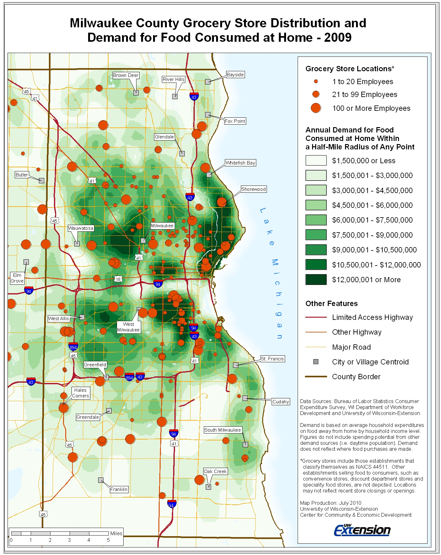
To map supply, a GIS can use business addresses and plot existing retail locations in a given NAICS retail category. Furthermore, the amount of consumer demand can be mapped using the demand calculations previously discussed in this section. Once mapped, the supply of retail locations can be shown along with the retail demand distribution.

The following map illustrates the use of GIS in examining the grocery store market in Milwaukee County, WI.  Here the locations of grocery stores (graduated symbols represent the size of each store) are overlaid on consumer spending demand (food consumed at home).  The map illustrates areas that are underserved (dark green demand and a lack of stores) as well as those well-served.

The combination of this information on the same map creates a powerful visual tool that can be used to analyze the downtown market. If the locations of retailers do not match the concentrations of consumer demand, a market gap may exist. If these gaps occur in or near a downtown or other business district, the maps could reveal opportunities for new retailers.

---

---

Program Updates

---

Latest Work